MY MODEL
This examples follows the model exposed in my Physics Undergraduate Thesis Project (2021-2022) whose code can be found GitHub repository.
The main equations of the model are the following:
Where
The configuration could be:
model = {
    "simulation": {
        "n_simulations": 100000,
        "n_executions": 1,
        "n_steps": 100
    },
    "compartments": {
        "Sh": { "initial_value": 0 },
        "S": {
            "initial_value": 1,
            "minus_compartments": "I"
        },
        "E": { "initial_value": 0 },
        "I": {
            "initial_value": "Io",
        },
        "R": { "initial_value": 0 },
        "Pd": { "initial_value": 0 },
        "D": { "initial_value": 0 },
    },
    "params": {
        "betta": {
            "min": 0.01,
            "max": 0.3,
            "min_limit": 0.01, // (1)
            "max_limit": 0.3
        },
        "Io": {
            "min": 1e-8,
            "max": 1e-5,
            "min_limit": 0,
            "max_limit": 1e-4
        },
        "phi": {
            "min": 0,
            "max": 0.5,
            "min_limit": 0,
            "max_limit": 1
        },
        "IFR": {
            "min":0.006,
            "max":0.014,
            "min_limit": 0.006,
            "max_limit": 0.014
        },
        "offset": {
            "type": "int", // (2)
            "min":5,
            "max":10,
            "min_limit": 0,
            "max_limit": 10
        }
    },
    "fixed_params": {
        "K_active": 12.4,
        "K_lockdown": 2.4,
        "sigma": 3.4,
        "mu": 1/4.2,
        "eta":1/5.2,
        "xi":1/10,
    },
    "reference": {
        "compartments" : ["D"],
        "offset": "offset" // (3)
    },
    "results": {
        "save_percentage": 0.5
    }
}
min_limitandmax_limitare the absolute limits in the automatic adjustment- This
offsetparameter will be used as an offset between the simulated data and the reference data - An offset can be applied to the reference while comparing it with the simulation data. Can be an interger or a parameter name defined in
params
Now we need to define the evolution function of the system and assign it to the model. In this case the evolution function is a lot more complicated than in previous examples.
Note: In case of complex problems like this it may be needed to write
[:]on values assignation.
import compartmental
compartmental.use_numpy()
# compartmental.use_cupy() # For GPU usage

MyModel = compartmental.GenericModel(model)

def evolve(m, time, p_active, *args, **kargs):
    ST = m.S + m.Sh
    sh = (1 - m.I) ** (m.sigma - 1)

    P_infection_active = 1- (1- m.betta * m.I) ** m.K_active
    P_infection_lockdown = 1- (1- m.betta * m.I) ** m.K_lockdown

    P_infection = p_active[time] * P_infection_active + (1-p_active[time]) * (1-sh*(1-m.phi)) * P_infection_lockdown


    m.Sh[:]    = ST * (1-p_active[time])*sh*(1-m.phi)
    delta_S = ST * P_infection
    m.S[:]     = (ST - m.Sh)  - delta_S

    m.D[:]     = m.xi * m.Pd
    m.R[:]     = m.mu * (1-m.IFR)  * m.I + m.R
    m.Pd[:]    = m.mu * m.IFR  * m.I + (1-m.xi) * m.Pd
    m.I[:]     = m.eta  * m.E + (1- m.mu) * m.I
    m.E[:]     = delta_S + (1-m.eta) * m.E

MyModel.evolve = evolve
For this example we will use a p_active defined as follows:
Once the model is defined and the evolution function is set we can create a trajectory of the model. We can set specific values for the random parameters as follows:
sample, sample_params = compartmental.util.get_model_sample_trajectory(
    MyModel, p_active,
    **{"betta": 0.13,
        "Io": 1e-6,
        "phi": 0.1,
        "IFR": 0.01,
        "offset": 8} # (1)
)

reference = numpy.copy(sample[MyModel.compartment_name_to_index["D"]])
offset is defined as the reference's offset in the model configuration.
Plotting the sample yields:
import matplotlib.pyplot as plt
list_of_sample_lines = []
_range = numpy.arange(model["simulation"]["n_steps"])

for s in sample:
    list_of_sample_lines.append(_range)
    list_of_sample_lines.append(s)
    list_of_sample_lines.append('-')

sample_lines = plt.plot(*list_of_sample_lines)
for line, compartment in zip(sample_lines, model["compartments"]):
    line.set_label(compartment)

plt.title("Compartments population evolution")
plt.xlabel("Time")
plt.ylabel("Population / Total")
plt.legend()
plt.show()

Now we can use the sample and try to infer the values of \(\beta\), \(Io\), \(\phi\), \(IFR\) and the offset:
ITERS = 15

# Main loop of adjustments:
# 1. Run
# 2. Read results
# 3. Compute weights
# 4. Adjuts configuration
for i in range(ITERS):
    MyModel.run(reference, f"my_model{i}.data", p_active)

    results = compartmental.util.load_parameters(f"my_model{i}.data")

    weights = numpy.exp(-2*results[0]/numpy.min(results[0]))

    compartmental.util.auto_adjust_model_params(MyModel, results, weights)


# Update for final photo with more simulations
MyModel.configuration.update({
    "simulation": {
        "n_simulations": 1000000,
        "n_executions": 4,
        "n_steps": 100
    },
    "results": {
        "save_percentage": 0.01
    }
})

MyModel.run(reference, "my_model.data", p_active)
Finnally we can plot the results:
results = compartmental.util.load_parameters("my_model.data")
weights = numpy.exp(-2*results[0]/numpy.min(results[0]))
weights /= numpy.min(weights)
percentiles = compartmental.util.get_percentiles_from_results(MyModel, results, 30, 70, weights, p_active, weights)
try:
# In case cupy is used
percentiles = percentiles.get()
sample = sample.get()
weights = weights.get()
results = results.get()
sample_params = sample_params.get()
except AttributeError:
pass
# Plot sample with a shadow of the results.
plt.figure()
plt.fill_between(numpy.arange(percentiles.shape[2]), percentiles[0,0], percentiles[0,2], alpha=0.3)
plt.xlabel("Simulation time")
plt.ylabel("Daily Deaths / Total population")
plt.plot(reference, 'black')
plt.plot(numpy.arange(percentiles.shape[2]), percentiles[0,1], '--', color='purple')
tax = plt.twinx()
tax.plot(p_active, ':', color='green')
tax.set_ylabel(r"$p(t)$")
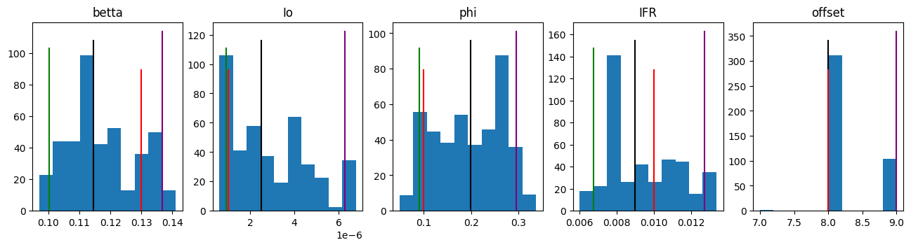
# Histograms with infered likelihood of the parameters
fig, *axes = plt.subplots(1, len(results)-1)
fig.set_figheight(3.5)
fig.set_figwidth(16)
for i, ax in enumerate(axes[0], 1):
_5, _50, _95 = compartmental.util.weighted_quantile(results[i], [5, 50, 95], weights)
for k, index in MyModel.param_to_index.items():
if index == i-1:
ax.set_title(k)
ax.hist(results[i], weights=weights)
ax.vlines(_5, *ax.get_ylim(), 'green')
ax.vlines(_50, *ax.get_ylim(), 'black')
ax.vlines(_95, *ax.get_ylim(), 'purple')
ax.vlines(sample_params[i-1], ax.get_ylim()[0], ax.get_ylim()[1]*3/4, 'red')
plt.show()