SEIR

\[ \begin{align} \nonumber \dot{S} &= -\beta \langle k \rangle \frac{I}{N}S. \\ \nonumber \dot{E} &= \beta \langle k \rangle \frac{I}{N}S - \eta E. \\ \nonumber \dot{I} &= \eta E - \mu I. \\ \nonumber \dot{R} &= \mu I. \end{align} \]

seir_model = {
    "simulation": { // (1)
        "n_simulations": 1000000, // (2)
        "n_executions": 1, // (3)
        "n_steps": 230 // (4)
    },
    "compartments": { // (5)
        "S": { 
            "initial_value": 1, // (6)
            "minus_compartments": "I" // (7)
        },
        "E": { "initial_value": 0 },
        "I": { 
            "initial_value": "Io", // (8)
        },
        "R": { "initial_value": 0 },
    },
    "params": { // (9)
        "betta": {
            "min": 0.1, // (10)
            "max": 0.3
        },
        "Io": {
            "min": 1e-6,
            "max": 1e-4
        }
    },
    "fixed_params": { // (11)
        "K_mean": 1,
        "mu": 0.07,
        "eta":0.08
    },
    "reference": { // (12)
        "compartments" : ["R"]
    },
    "results": { 
        "save_percentage": 0.01 // (13)
    }
}

1. Here we define simulation parameters
2. How many simulations to do in parallel each execution
3. Number of times the simulation runs

4. Number of times the evolution function is executed each simulation

5. Here we define the compartments of the model. Each field must be unique

6. Initial value set to a fixed number
7. You subtract the value of other compartments after all of them are initialized

8. You can set the initial value of compartments as parameters

9. Here we define parameters that will be randomly generated for each simulation. Each field must be unique

10. A min value and max value must be set for each parameter

11. Definition of constant for all the simulations

12. Definition of which compartments the results should be compared with

13. Percentage of simulations that will be saved. The best of course

Now we need to define the evolution function of the system and assign it to the model:

import compartmental as gcm
gcm.use_numpy()
# gcm.use_cupy() # For GPU usage

SeirModel = gcm.GenericModel(seir_model)

def evolve(m, *args, **kargs):
    p_infected = m.betta * m.K_mean * m.I

    m.R += m.mu * m.I
    m.I += m.E * m.eta - m.I * m.mu
    m.E += m.S * p_infected - m.E * m.eta
    m.S -= m.S * p_infected

SeirModel.evolve = evolve

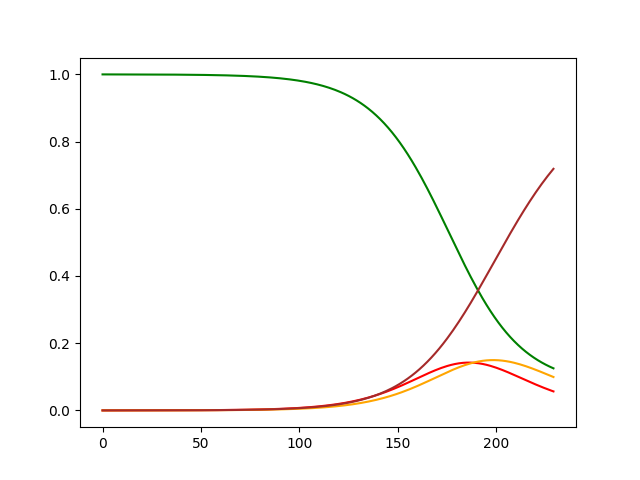
Once the model is defined and the evolution function is set we can create a trajectory of the model. We can set specific values for the random parameters as follows:

sample, sample_params = gcm.util.get_model_sample_trajectory(
    SeirModel, 
    **{"betta": 0.2, "Io":6e-5}
)

Plotting the sample yields:

import matplotlib.pyplot as plt
plt.plot(sample[SeirModel.compartment_name_to_index["S"]], 'green')
plt.plot(sample[SeirModel.compartment_name_to_index["E"]], 'red')
plt.plot(sample[SeirModel.compartment_name_to_index["I"]], 'orange')
plt.plot(sample[SeirModel.compartment_name_to_index["R"]], 'brown')
plt.show()

---

Now we can use the sample and try to infer the values of \(\beta\) and \(Io\).

SeirModel.run(sample[SeirModel.compartment_name_to_index["R"]], "seir.data")

The results are save in the seir.data file. We load them, compute the weights and the percentiles 30 and 70 with:

results = gcm.util.load_parameters("seir.data")
weights = numpy.exp(-results[0]/numpy.min(results[0]))

percentiles = gcm.util.get_percentiles_from_results(SeirModel, results, 30, 70)

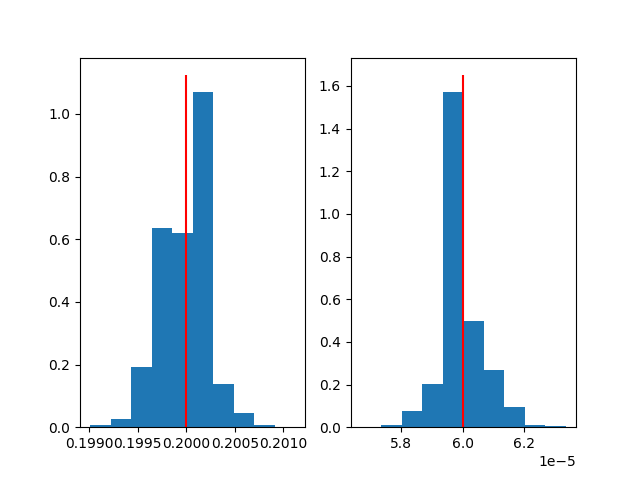
Finally plot the reference values with the percentiles and histograms for the parameters \(\beta\) and \(Io\) (the red line indicates the value used for the reference):

plt.figure()
plt.fill_between(numpy.arange(percentiles.shape[2]), percentiles[0,0], percentiles[0,2], alpha=0.3)
plt.plot(sample[SeirModel.compartment_name_to_index["R"]], 'black')
plt.plot(numpy.arange(percentiles.shape[2]), percentiles[0,1], '--', color='purple')

fig, *axes = plt.subplots(1, len(results)-1)
for i, ax in enumerate(axes[0], 1):
    ax.hist(results[i], weights=weights)
    ax.vlines(sample_params[i-1], *ax.get_ylim(), 'red')

plt.show()